三言两语讲完了反向传播,一个公式也没有,果然是面向“懒惰工程师”的快餐教程。比较喜欢“不提神经元,我们不是巫婆”的观点。这次不需要自己写算法,直接上TensorFlow了。
任务 2: 随机梯度下降
使用梯度下降和随机梯度下降训练一个全连接网络。
安装TensorFlow

新MacBookPro都是A卡,不用想cuda了,只能CPU。忍不住要黑:


Mac OS X Python 3.5 下的安装方法:
easy_install --upgrade six
export TF_BINARY_URL=https://storage.googleapis.com/tensorflow/mac/cpu/tensorflow-0.11.0-py3-none-any.whl
pip3 install --upgrade $TF_BINARY_URL
不要像官网那样用sudo,那不是pip的正确使用方式。
测试TensorFlow
python3
Python 3.5.2 (default, Sep 15 2016, 07:38:42)
[GCC 4.2.1 Compatible Apple LLVM 7.3.0 (clang-703.0.31)] on darwin
Type "help", "copyright", "credits" or "license" for more information.
>>> import tensorflow as tf
>>> hello = tf.constant('Hello, TensorFlow!')
>>> sess = tf.Session()
>>> print(sess.run(hello))
b'Hello, TensorFlow!'
>>> a = tf.constant(10)
>>> b = tf.constant(32)
>>> print(sess.run(a + b))
42
TensorFlow入门
TensorFlow的工作流程像一张图,先创建图,并在图上定义一些常量、变量和类似于函数的东西。如果熟悉OpenGL的话,肯定会觉得这有点像shader编程,我们在TF里写了段程序。
graph = tf.Graph()
with graph.as_default():
    ...
然后在图上创建一个session,意思就是我要调用刚才写的程序了
with tf.Session(graph=graph) as session:
    ...
第一次任务是用梯度下降训练一个非正则化的多项式逻辑斯谛回归,整个训练代码谷歌都给出了,注释也很详尽:
# With gradient descent training, even this much data is prohibitive.
# Subset the training data for faster turnaround.
train_subset = 10000

graph = tf.Graph()
with graph.as_default():
    # Input data.
    # Load the training, validation and test data into constants that are
    # attached to the graph.
    tf_train_dataset = tf.constant(train_dataset[:train_subset, :])
    tf_train_labels = tf.constant(train_labels[:train_subset])
    tf_valid_dataset = tf.constant(valid_dataset)
    tf_test_dataset = tf.constant(test_dataset)

    # Variables.
    # These are the parameters that we are going to be training. The weight
    # matrix will be initialized using random values following a (truncated)
    # normal distribution. The biases get initialized to zero.
    weights = tf.Variable(
        tf.truncated_normal([image_size * image_size, num_labels]))
    biases = tf.Variable(tf.zeros([num_labels]))

    # Training computation.
    # We multiply the inputs with the weight matrix, and add biases. We compute
    # the softmax and cross-entropy (it's one operation in TensorFlow, because
    # it's very common, and it can be optimized). We take the average of this
    # cross-entropy across all training examples: that's our loss.
    logits = tf.matmul(tf_train_dataset, weights) + biases
    loss = tf.reduce_mean(
        tf.nn.softmax_cross_entropy_with_logits(logits, tf_train_labels))

    # Optimizer.
    # We are going to find the minimum of this loss using gradient descent.
    optimizer = tf.train.GradientDescentOptimizer(0.5).minimize(loss)

    # Predictions for the training, validation, and test data.
    # These are not part of training, but merely here so that we can report
    # accuracy figures as we train.
    train_prediction = tf.nn.softmax(logits)
    valid_prediction = tf.nn.softmax(
        tf.matmul(tf_valid_dataset, weights) + biases)
    test_prediction = tf.nn.softmax(tf.matmul(tf_test_dataset, weights) + biases)

num_steps = 801


def accuracy(predictions, labels):
    return (100.0 * np.sum(np.argmax(predictions, 1) == np.argmax(labels, 1))
            / predictions.shape[0])


with tf.Session(graph=graph) as session:
    # This is a one-time operation which ensures the parameters get initialized as
    # we described in the graph: random weights for the matrix, zeros for the
    # biases.
    tf.initialize_all_variables().run()
    print('Initialized')
    for step in range(num_steps):
        # Run the computations. We tell .run() that we want to run the optimizer,
        # and get the loss value and the training predictions returned as numpy
        # arrays.
        _, l, predictions = session.run([optimizer, loss, train_prediction])
        if (step % 100 == 0):
            print('Loss at step %d: %f' % (step, l))
            print('Training accuracy: %.1f%%' % accuracy(
                predictions, train_labels[:train_subset, :]))
            # Calling .eval() on valid_prediction is basically like calling run(), but
            # just to get that one numpy array. Note that it recomputes all its graph
            # dependencies.
            print('Validation accuracy: %.1f%%' % accuracy(
                valid_prediction.eval(), valid_labels))
    print('Test accuracy: %.1f%%' % accuracy(test_prediction.eval(), test_labels))
注意官方代码中的
tf.global_variables_initializer().run()
在tensorflow-0.11.0中会抛出:
Traceback (most recent call last):
  File "udacity-deep-learning/2_fullyconnected.py", line 142, in <module>
    tf.global_variables_initializer().run()
AttributeError: module 'tensorflow' has no attribute 'global_variables_initializer'
需要修改为
tf.initialize_all_variables().run()
运行后得到:
Loss at step 800: 1.066299
Training accuracy: 79.6%
Validation accuracy: 75.0%
Test accuracy: 83.0%
注意到这里的训练规模是
# With gradient descent training, even this much data is prohibitive.
# Subset the training data for faster turnaround.
train_subset = 10000
因为梯度下降实在太慢了,改用随机梯度下降会快一些,相较于上一版代码,只不过在每一个迭代中随机选取了部分实例用于训练:
with tf.Session(graph=graph) as session:
  tf.global_variables_initializer().run()
  print("Initialized")
  for step in range(num_steps):
    # Pick an offset within the training data, which has been randomized.
    # Note: we could use better randomization across epochs.
    offset = (step * batch_size) % (train_labels.shape[0] - batch_size)
    # Generate a minibatch.
    batch_data = train_dataset[offset:(offset + batch_size), :]
    batch_labels = train_labels[offset:(offset + batch_size), :]
    # Prepare a dictionary telling the session where to feed the minibatch.
    # The key of the dictionary is the placeholder node of the graph to be fed,
    # and the value is the numpy array to feed to it.
    feed_dict = {tf_train_dataset : batch_data, tf_train_labels : batch_labels}
    _, l, predictions = session.run(
      [optimizer, loss, train_prediction], feed_dict=feed_dict)
得到
Minibatch loss at step 3000: 1.182136
Minibatch accuracy: 75.0%
Validation accuracy: 79.0%
Test accuracy: 86.6%
训练了更多迭代,accuracy上升了不少,用时却减少了很多。
题目
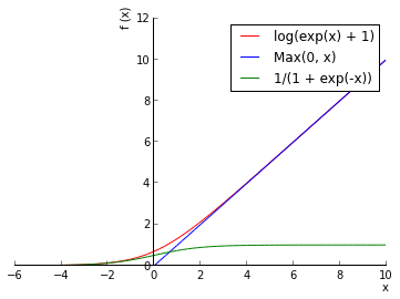
请在上述代码的基础上将其改造为使用ReLU激活函数f(x)=max(0,x):

1024个隐藏层节点的神经网络。
batch_size = 128
hidden_size = 1024

graph = tf.Graph()
with graph.as_default():
    # Input data. For the training data, we use a placeholder that will be fed
    # at run time with a training minibatch.
    tf_train_dataset = tf.placeholder(tf.float32,
                                      shape=(batch_size, image_size * image_size))
    tf_train_labels = tf.placeholder(tf.float32, shape=(batch_size, num_labels))
    tf_valid_dataset = tf.constant(valid_dataset)
    tf_test_dataset = tf.constant(test_dataset)

    # Variables.
    W1 = tf.Variable(tf.truncated_normal([image_size * image_size, hidden_size]))
    b1 = tf.Variable(tf.zeros([hidden_size]))

    W2 = tf.Variable(tf.truncated_normal([hidden_size, num_labels]))
    b2 = tf.Variable(tf.zeros([num_labels]))

    # Training computation.
    y1 = tf.nn.relu(tf.matmul(tf_train_dataset, W1) + b1)
    logits = tf.matmul(y1, W2) + b2

    loss = tf.reduce_mean(
        tf.nn.softmax_cross_entropy_with_logits(logits, tf_train_labels))

    # Optimizer.
    optimizer = tf.train.GradientDescentOptimizer(0.5).minimize(loss)

    # Predictions for the training, validation, and test data.
    train_prediction = tf.nn.softmax(logits)

    y1_valid = tf.nn.relu(tf.matmul(tf_valid_dataset, W1) + b1)
    valid_logits = tf.matmul(y1_valid, W2) + b2
    valid_prediction = tf.nn.softmax(valid_logits)

    y1_test = tf.nn.relu(tf.matmul(tf_test_dataset, W1) + b1)
    test_logits = tf.matmul(y1_test, W2) + b2
    test_prediction = tf.nn.softmax(test_logits)

# Let's run it:
num_steps = 3001

with tf.Session(graph=graph) as session:
    tf.initialize_all_variables().run()
    print("Initialized")
    for step in range(num_steps):
        # Pick an offset within the training data, which has been randomized.
        # Note: we could use better randomization across epochs.
        offset = (step * batch_size) % (train_labels.shape[0] - batch_size)
        # Generate a minibatch.
        batch_data = train_dataset[offset:(offset + batch_size), :]
        batch_labels = train_labels[offset:(offset + batch_size), :]
        # Prepare a dictionary telling the session where to feed the minibatch.
        # The key of the dictionary is the placeholder node of the graph to be fed,
        # and the value is the numpy array to feed to it.
        feed_dict = {tf_train_dataset: batch_data, tf_train_labels: batch_labels}
        _, l, predictions = session.run(
            [optimizer, loss, train_prediction], feed_dict=feed_dict)
        if (step % 500 == 0):
            print("Minibatch loss at step %d: %f" % (step, l))
            print("Minibatch accuracy: %.1f%%" % accuracy(predictions, batch_labels))
            print("Validation accuracy: %.1f%%" % accuracy(
                valid_prediction.eval(), valid_labels))
    print("Test accuracy: %.1f%%" % accuracy(test_prediction.eval(), test_labels))
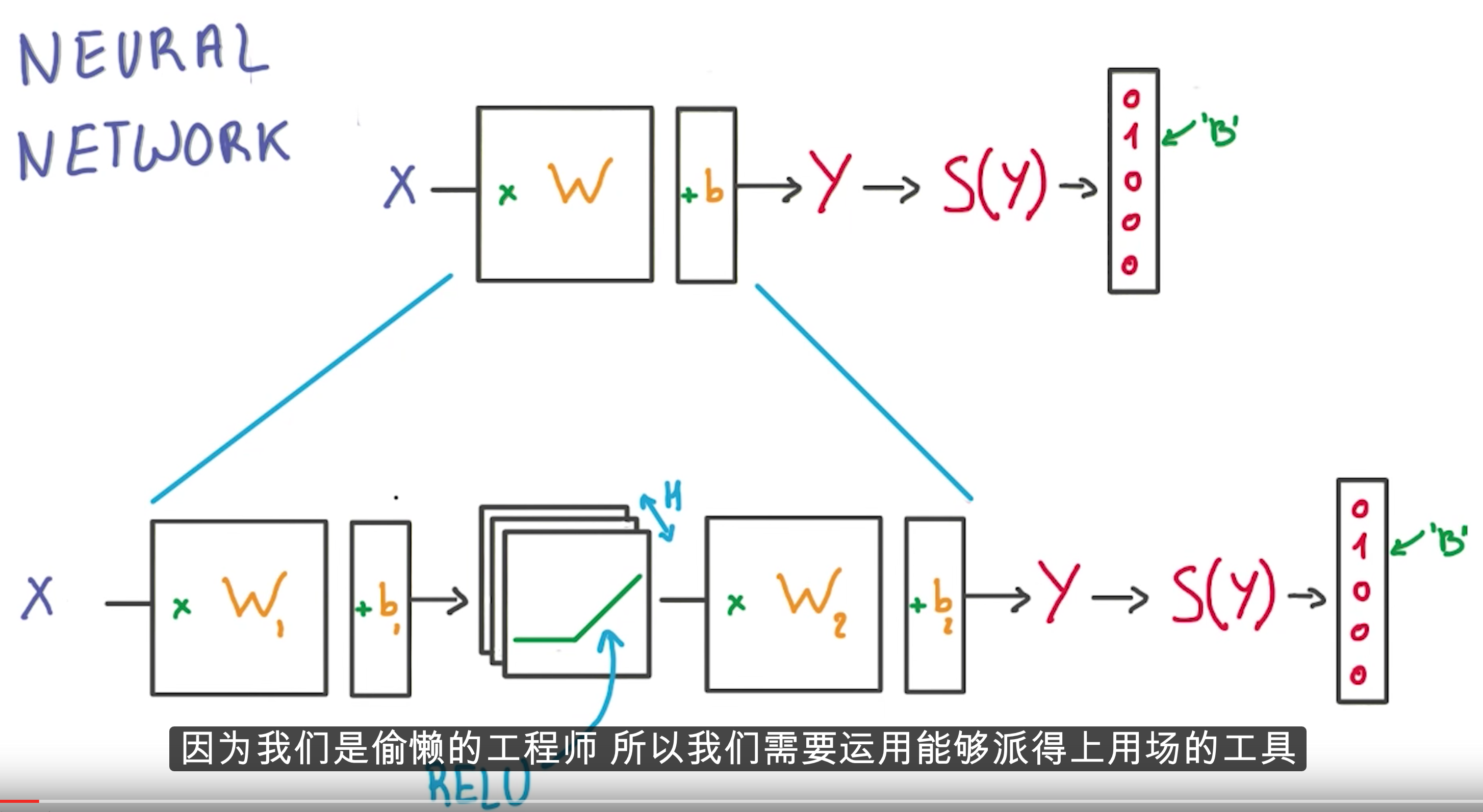
两者的主要区别是,

逻辑斯谛回归:
    weights = tf.Variable(tf.truncated_normal([image_size * image_size, num_labels]))
    biases = tf.Variable(tf.zeros([num_labels]))
    logits = tf.matmul(tf_train_dataset, weights) + biases
    loss = tf.reduce_mean(tf.nn.softmax_cross_entropy_with_logits(logits, tf_train_labels))
神经网络:
    # Variables.
    W1 = tf.Variable(tf.truncated_normal([image_size * image_size, hidden_size]))
    b1 = tf.Variable(tf.zeros([hidden_size]))

    W2 = tf.Variable(tf.truncated_normal([hidden_size, num_labels]))
    b2 = tf.Variable(tf.zeros([num_labels]))

    # Training computation.
    y1 = tf.nn.relu(tf.matmul(tf_train_dataset, W1) + b1)
    logits = tf.matmul(y1, W2) + b2

    loss = tf.reduce_mean(tf.nn.softmax_cross_entropy_with_logits(logits, tf_train_labels))
于是一个线性模型就进化为非线性的神经网络。
这一步得到:
Minibatch loss at step 3000: 1.465061
Minibatch accuracy: 83.6%
Validation accuracy: 81.4%
Test accuracy: 88.6%
由于随机数的因素,最终结果可能会有少许波动,但总体还是优于逻辑斯谛回归的。
 码农场
码农场
机器要跟得上