这次的看点是怎么在TensorFlow里实现正则化、dropout和学习率递减的技巧;顺便演示了下自动调参。

任务 3: 正则化
使用正则化去优化深度学习模型
题目1
给上次练习实现的逻辑斯谛回归和神经网络加上L2正则,检查性能提升。
逻辑斯谛回归
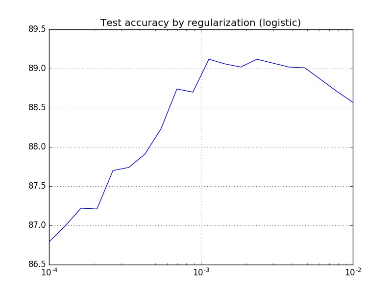
对于beta这个超参数的取值,用一段自动调参的脚本在一个区间内遍历搜索:
beta_val = np.logspace(-4, -2, 20)
accuracy_val = []

# logistic model
batch_size = 128

graph = tf.Graph()
with graph.as_default():
    # Input data. For the training data, we use a placeholder that will be fed
    # at run time with a training minibatch.
    tf_train_dataset = tf.placeholder(tf.float32,
                                      shape=(batch_size, image_size * image_size))
    tf_train_labels = tf.placeholder(tf.float32, shape=(batch_size, num_labels))
    tf_valid_dataset = tf.constant(valid_dataset)
    tf_test_dataset = tf.constant(test_dataset)
    beta_regul = tf.placeholder(tf.float32)

    # Variables.
    weights = tf.Variable(tf.truncated_normal([image_size * image_size, num_labels]))
    biases = tf.Variable(tf.zeros([num_labels]))

    # Training computation.
    logits = tf.matmul(tf_train_dataset, weights) + biases
    loss = tf.reduce_mean(
        tf.nn.softmax_cross_entropy_with_logits(logits, tf_train_labels)) + beta_regul * tf.nn.l2_loss(weights)

    # Optimizer.
    optimizer = tf.train.GradientDescentOptimizer(0.5).minimize(loss)

    # Predictions for the training, validation, and test data.
    train_prediction = tf.nn.softmax(logits)
    valid_prediction = tf.nn.softmax(tf.matmul(tf_valid_dataset, weights) + biases)
    test_prediction = tf.nn.softmax(tf.matmul(tf_test_dataset, weights) + biases)

num_steps = 3001

for beta in beta_val:
    with tf.Session(graph=graph) as session:
        tf.initialize_all_variables().run()
        for step in range(num_steps):
            # Pick an offset within the training data, which has been randomized.
            # Note: we could use better randomization across epochs.
            offset = (step * batch_size) % (train_labels.shape[0] - batch_size)
            # Generate a minibatch.
            batch_data = train_dataset[offset:(offset + batch_size), :]
            batch_labels = train_labels[offset:(offset + batch_size), :]
            # Prepare a dictionary telling the session where to feed the minibatch.
            # The key of the dictionary is the placeholder node of the graph to be fed,
            # and the value is the numpy array to feed to it.
            feed_dict = {tf_train_dataset: batch_data, tf_train_labels: batch_labels, beta_regul: beta}
            _, l, predictions = session.run([optimizer, loss, train_prediction], feed_dict=feed_dict)
            # if (step % 500 == 0):
            #     print("Minibatch loss at step %d: %f" % (step, l))
            #     print("Minibatch accuracy: %.1f%%" % accuracy(predictions, batch_labels))
            #     print("Validation accuracy: %.1f%%" % accuracy(valid_prediction.eval(), valid_labels))
        print("L2 regularization(beta=%.5f) Test accuracy: %.1f%%" % (
            beta, accuracy(test_prediction.eval(), test_labels)))

        accuracy_val.append(accuracy(test_prediction.eval(), test_labels))

print('Best beta=%f, accuracy=%.1f%%' % (beta_val[np.argmax(accuracy_val)], max(accuracy_val)))
plt.semilogx(beta_val, accuracy_val)
plt.grid(True)
plt.title('Test accuracy by regularization (logistic)')
plt.show()
输出
L2 regularization(beta=0.00010) Test accuracy: 86.8%
L2 regularization(beta=0.00013) Test accuracy: 87.0%
L2 regularization(beta=0.00016) Test accuracy: 87.2%
L2 regularization(beta=0.00021) Test accuracy: 87.2%
L2 regularization(beta=0.00026) Test accuracy: 87.7%
L2 regularization(beta=0.00034) Test accuracy: 87.7%
L2 regularization(beta=0.00043) Test accuracy: 87.9%
L2 regularization(beta=0.00055) Test accuracy: 88.2%
L2 regularization(beta=0.00070) Test accuracy: 88.7%
L2 regularization(beta=0.00089) Test accuracy: 88.7%
L2 regularization(beta=0.00113) Test accuracy: 89.1%
L2 regularization(beta=0.00144) Test accuracy: 89.1%
L2 regularization(beta=0.00183) Test accuracy: 89.0%
L2 regularization(beta=0.00234) Test accuracy: 89.1%
L2 regularization(beta=0.00298) Test accuracy: 89.1%
L2 regularization(beta=0.00379) Test accuracy: 89.0%
L2 regularization(beta=0.00483) Test accuracy: 89.0%
L2 regularization(beta=0.00616) Test accuracy: 88.9%
L2 regularization(beta=0.00785) Test accuracy: 88.7%
L2 regularization(beta=0.01000) Test accuracy: 88.6%
Best beta=0.001129, accuracy=89.1%
可视化

神经网络模型
用类似的手法
# NN model
batch_size = 128
hidden_size = 1024

graph = tf.Graph()
with graph.as_default():
    # Input data. For the training data, we use a placeholder that will be fed
    # at run time with a training minibatch.
    tf_train_dataset = tf.placeholder(tf.float32, shape=(batch_size, image_size * image_size))
    tf_train_labels = tf.placeholder(tf.float32, shape=(batch_size, num_labels))
    tf_valid_dataset = tf.constant(valid_dataset)
    tf_test_dataset = tf.constant(test_dataset)
    tf_beta = tf.placeholder(tf.float32)

    # Variables.
    W1 = tf.Variable(tf.truncated_normal([image_size * image_size, hidden_size]))
    b1 = tf.Variable(tf.zeros([hidden_size]))

    W2 = tf.Variable(tf.truncated_normal([hidden_size, num_labels]))
    b2 = tf.Variable(tf.zeros([num_labels]))

    # Training computation.
    y1 = tf.nn.relu(tf.matmul(tf_train_dataset, W1) + b1)
    logits = tf.matmul(y1, W2) + b2

    loss = tf.reduce_mean(tf.nn.softmax_cross_entropy_with_logits(logits, tf_train_labels))

    loss = loss + tf_beta * (tf.nn.l2_loss(W1) + tf.nn.l2_loss(b1) + tf.nn.l2_loss(W2) + tf.nn.l2_loss(b2))

    # Optimizer.
    optimizer = tf.train.GradientDescentOptimizer(0.5).minimize(loss)

    # Predictions for the training, validation, and test data.
    train_prediction = tf.nn.softmax(logits)

    y1_valid = tf.nn.relu(tf.matmul(tf_valid_dataset, W1) + b1)
    valid_logits = tf.matmul(y1_valid, W2) + b2
    valid_prediction = tf.nn.softmax(valid_logits)

    y1_test = tf.nn.relu(tf.matmul(tf_test_dataset, W1) + b1)
    test_logits = tf.matmul(y1_test, W2) + b2
    test_prediction = tf.nn.softmax(test_logits)

# Let's run it:
num_steps = 3001

accuracy_val.clear()
for beta in np.logspace(-4, -2, 20):
    with tf.Session(graph=graph) as session:
        tf.initialize_all_variables().run()
        # print("Initialized")
        for step in range(num_steps):
            # Pick an offset within the training data, which has been randomized.
            # Note: we could use better randomization across epochs.
            offset = (step * batch_size) % (train_labels.shape[0] - batch_size)
            # Generate a minibatch.
            batch_data = train_dataset[offset:(offset + batch_size), :]
            batch_labels = train_labels[offset:(offset + batch_size), :]
            # Prepare a dictionary telling the session where to feed the minibatch.
            # The key of the dictionary is the placeholder node of the graph to be fed,
            # and the value is the numpy array to feed to it.
            feed_dict = {tf_train_dataset: batch_data, tf_train_labels: batch_labels, tf_beta: beta}
            _, l, predictions = session.run([optimizer, loss, train_prediction], feed_dict=feed_dict)
            # if (step % 500 == 0):
            #     print("Minibatch loss at step %d: %f" % (step, l))
            #     print("Minibatch accuracy: %.1f%%" % accuracy(predictions, batch_labels))
            #     print("Validation accuracy: %.1f%%" % accuracy(valid_prediction.eval(), valid_labels))
        print("L2 regularization(beta=%.5f) Test accuracy: %.1f%%" % (
            beta, accuracy(test_prediction.eval(), test_labels)))
        accuracy_val.append(accuracy(test_prediction.eval(), test_labels))

print('Best beta=%f, accuracy=%.1f%%' % (beta_val[np.argmax(accuracy_val)], max(accuracy_val)))
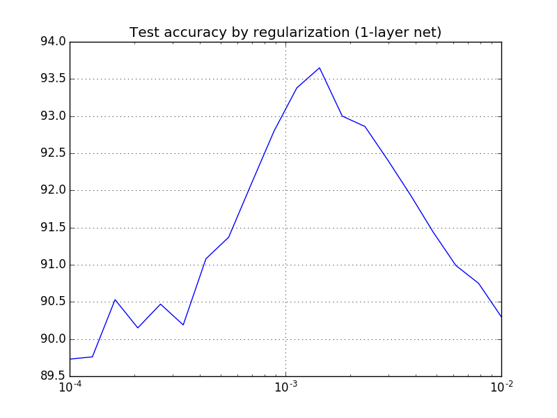
plt.semilogx(beta_val, accuracy_val)
plt.grid(True)
plt.title('Test accuracy by regularization (1-layer net)')
plt.show()
输出
L2 regularization(beta=0.00010) Test accuracy: 89.7%
L2 regularization(beta=0.00013) Test accuracy: 89.8%
L2 regularization(beta=0.00016) Test accuracy: 90.5%
L2 regularization(beta=0.00021) Test accuracy: 90.2%
L2 regularization(beta=0.00026) Test accuracy: 90.5%
L2 regularization(beta=0.00034) Test accuracy: 90.2%
L2 regularization(beta=0.00043) Test accuracy: 91.1%
L2 regularization(beta=0.00055) Test accuracy: 91.4%
L2 regularization(beta=0.00070) Test accuracy: 92.1%
L2 regularization(beta=0.00089) Test accuracy: 92.8%
L2 regularization(beta=0.00113) Test accuracy: 93.4%
L2 regularization(beta=0.00144) Test accuracy: 93.7%
L2 regularization(beta=0.00183) Test accuracy: 93.0%
L2 regularization(beta=0.00234) Test accuracy: 92.9%
L2 regularization(beta=0.00298) Test accuracy: 92.4%
L2 regularization(beta=0.00379) Test accuracy: 91.9%
L2 regularization(beta=0.00483) Test accuracy: 91.4%
L2 regularization(beta=0.00616) Test accuracy: 91.0%
L2 regularization(beta=0.00785) Test accuracy: 90.8%
L2 regularization(beta=0.01000) Test accuracy: 90.3%
Best beta=0.001438, accuracy=93.7%
最佳beta是0.001438,我们可以将这个值用于接下来的试验。
可视化

事实上,上面只是追求test分数好看而已,应该在开发集上选择参数。《CS229编程5:正则化线性回归与偏差方差权衡》才是正确做法。
题目2:过拟合
将训练集减小到batch数目的几倍,看看会发生什么。
few_batch_size = batch_size * 5
small_train_dataset = train_dataset[:few_batch_size, :]
small_train_labels = train_labels[:few_batch_size, :]

print('Training set', small_train_dataset.shape, small_train_labels.shape)

num_steps = 3001

with tf.Session(graph=graph) as session:
    tf.initialize_all_variables().run()
    print("Initialized")
    for step in range(num_steps):
        # Pick an offset within the training data, which has been randomized.
        # Note: we could use better randomization across epochs.
        offset = (step * batch_size) % (small_train_labels.shape[0] - batch_size)
        # Generate a minibatch.
        batch_data = small_train_dataset[offset:(offset + batch_size), :]
        batch_labels = small_train_labels[offset:(offset + batch_size), :]
        # Prepare a dictionary telling the session where to feed the minibatch.
        # The key of the dictionary is the placeholder node of the graph to be fed,
        # and the value is the numpy array to feed to it.
        feed_dict = {tf_train_dataset: batch_data, tf_train_labels: batch_labels, tf_beta: 0.001438}
        _, l, predictions = session.run(
            [optimizer, loss, train_prediction], feed_dict=feed_dict)
        if (step % 500 == 0):
            print("Minibatch loss at step %d: %f" % (step, l))
            print("Minibatch accuracy: %.1f%%" % accuracy(predictions, batch_labels))
            print("Validation accuracy: %.1f%%" % accuracy(
                valid_prediction.eval(), valid_labels))
    print("Overfitting with small dataset Test accuracy: %.1f%%" % accuracy(test_prediction.eval(), test_labels))
输出
Training set (640, 784) (640, 10)
Overfitting with small dataset Test accuracy: 84.5%
跌了很多,当然的。
题目3:Dropout
引入Dropout技巧,看看性能提升,以及能否改善上面的过拟合。
改善性能
batch_size = 128
hidden_size = 1024

graph = tf.Graph()
with graph.as_default():
    # Input data. For the training data, we use a placeholder that will be fed
    # at run time with a training minibatch.
    tf_train_dataset = tf.placeholder(tf.float32, shape=(batch_size, image_size * image_size))
    tf_train_labels = tf.placeholder(tf.float32, shape=(batch_size, num_labels))
    tf_valid_dataset = tf.constant(valid_dataset)
    tf_test_dataset = tf.constant(test_dataset)
    tf_beta = tf.placeholder(tf.float32)

    # Variables.
    W1 = tf.Variable(tf.truncated_normal([image_size * image_size, hidden_size]))
    b1 = tf.Variable(tf.zeros([hidden_size]))

    W2 = tf.Variable(tf.truncated_normal([hidden_size, num_labels]))
    b2 = tf.Variable(tf.zeros([num_labels]))

    # Training computation.
    y1 = tf.nn.relu(tf.matmul(tf_train_dataset, W1) + b1)
    y1 = tf.nn.dropout(y1, 0.5)  # Dropout
    logits = tf.matmul(y1, W2) + b2

    loss = tf.reduce_mean(tf.nn.softmax_cross_entropy_with_logits(logits, tf_train_labels))

    loss = loss + tf_beta * (tf.nn.l2_loss(W1) + tf.nn.l2_loss(b1) + tf.nn.l2_loss(W2) + tf.nn.l2_loss(b2))

    # Optimizer.
    optimizer = tf.train.GradientDescentOptimizer(0.5).minimize(loss)

    # Predictions for the training, validation, and test data.
    train_prediction = tf.nn.softmax(logits)

    y1_valid = tf.nn.relu(tf.matmul(tf_valid_dataset, W1) + b1)
    valid_logits = tf.matmul(y1_valid, W2) + b2
    valid_prediction = tf.nn.softmax(valid_logits)

    y1_test = tf.nn.relu(tf.matmul(tf_test_dataset, W1) + b1)
    test_logits = tf.matmul(y1_test, W2) + b2
    test_prediction = tf.nn.softmax(test_logits)

# Let's run it:
num_steps = 3001

with tf.Session(graph=graph) as session:
    tf.initialize_all_variables().run()
    print("Initialized")
    for step in range(num_steps):
        # Pick an offset within the training data, which has been randomized.
        # Note: we could use better randomization across epochs.
        offset = (step * batch_size) % (train_labels.shape[0] - batch_size)
        # Generate a minibatch.
        batch_data = train_dataset[offset:(offset + batch_size), :]
        batch_labels = train_labels[offset:(offset + batch_size), :]
        # Prepare a dictionary telling the session where to feed the minibatch.
        # The key of the dictionary is the placeholder node of the graph to be fed,
        # and the value is the numpy array to feed to it.
        feed_dict = {tf_train_dataset: batch_data, tf_train_labels: batch_labels, tf_beta: 0.001438}
        _, l, predictions = session.run([optimizer, loss, train_prediction], feed_dict=feed_dict)
        if (step % 500 == 0):
            print("Minibatch loss at step %d: %f" % (step, l))
            print("Minibatch accuracy: %.1f%%" % accuracy(predictions, batch_labels))
            print("Validation accuracy: %.1f%%" % accuracy(
                valid_prediction.eval(), valid_labels))
    print("Dropout Test accuracy: %.1f%%" % accuracy(test_prediction.eval(), test_labels))
唯一的改动是调用了一次dropout:
y1 = tf.nn.dropout(y1, 0.5) # Dropout

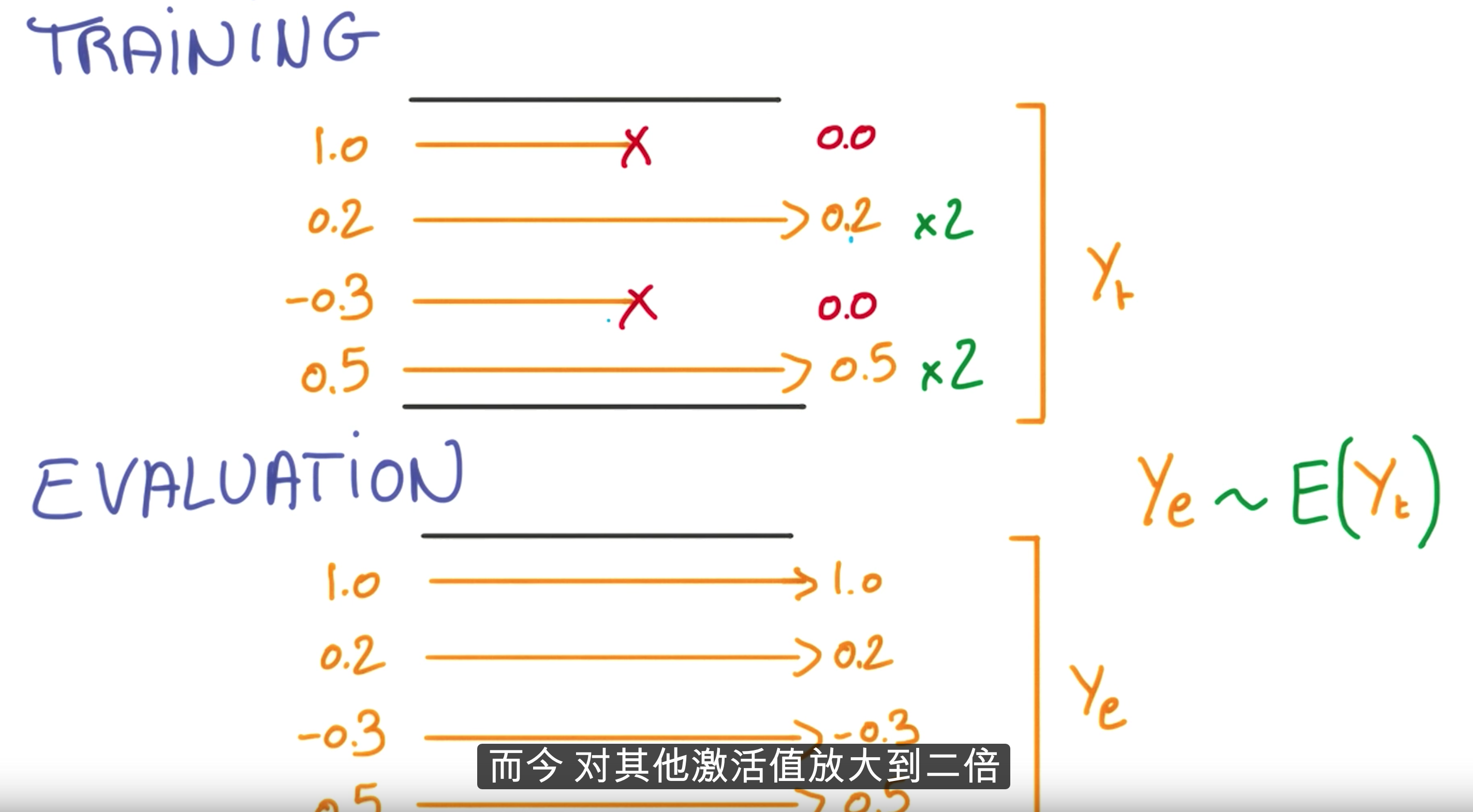
该方法会自动缩放倍数,所以不用操心:
With probability keep_prob, outputs the input element scaled up by 1 / keep_prob, otherwise outputs 0. The scaling is so that the expected sum is unchanged.
输出
Dropout Test accuracy: 92.3%
改善过拟合
Dropout with small dataset Test accuracy: 86.1%
的确有所回升。
题目4:深度神经网络
上面1-layer(指的是隐藏层)神经网络并不稀奇,Python版的matlab版的Java版的满大街都是,并不能发挥TF的全力,试试multi-layer如何?还可以尝试学习率递减的策略。
那就不客气了,来个3-layer,迭代数目也4倍:
batch_size = 128
fc1_size = 4096
fc2_size = 2048
fc3_size = 128

graph = tf.Graph()
with graph.as_default():
    # Input data. For the training data, we use a placeholder that will be fed
    # at run time with a training minibatch.
    tf_train_dataset = tf.placeholder(tf.float32,
                                      shape=(batch_size, image_size * image_size))
    tf_train_labels = tf.placeholder(tf.float32, shape=(batch_size, num_labels))
    tf_valid_dataset = tf.constant(valid_dataset)
    tf_test_dataset = tf.constant(test_dataset)
    tf_beta = tf.placeholder(tf.float32)
    global_step = tf.Variable(0)  # count the number of steps taken.

    # Variables.
    # stddev is very important!!!
    W1 = tf.Variable(
        tf.truncated_normal([image_size * image_size, fc1_size], stddev=np.sqrt(2.0 / (image_size * image_size))))
    b1 = tf.Variable(tf.zeros([fc1_size]))

    W2 = tf.Variable(tf.truncated_normal([fc1_size, fc2_size], stddev=np.sqrt(2.0 / fc1_size)))
    b2 = tf.Variable(tf.zeros([fc2_size]))

    W3 = tf.Variable(tf.truncated_normal([fc2_size, fc3_size], stddev=np.sqrt(2.0 / fc2_size)))
    b3 = tf.Variable(tf.zeros([fc3_size]))

    W4 = tf.Variable(tf.truncated_normal([fc3_size, num_labels], stddev=np.sqrt(2.0 / fc3_size)))
    b4 = tf.Variable(tf.zeros([num_labels]))

    # Training computation.
    y1 = tf.nn.relu(tf.matmul(tf_train_dataset, W1) + b1)
    # y1 = tf.nn.dropout(y1, 0.5)

    y2 = tf.nn.relu(tf.matmul(y1, W2) + b2)
    # y2 = tf.nn.dropout(y2, 0.5)

    y3 = tf.nn.relu(tf.matmul(y2, W3) + b3)
    # y3 = tf.nn.dropout(y3, 0.5)

    logits = tf.matmul(y3, W4) + b4

    loss = tf.reduce_mean(
        tf.nn.softmax_cross_entropy_with_logits(logits, tf_train_labels))

    loss = loss + tf_beta * (tf.nn.l2_loss(W1) + tf.nn.l2_loss(b1) + tf.nn.l2_loss(W2) + tf.nn.l2_loss(b2) +
                             tf.nn.l2_loss(W3) + tf.nn.l2_loss(b3) + tf.nn.l2_loss(W4) + tf.nn.l2_loss(b4))

    # Optimizer
    learning_rate = tf.train.exponential_decay(0.5, global_step, 1000, 0.7, staircase=True)
    optimizer = tf.train.GradientDescentOptimizer(learning_rate).minimize(loss, global_step=global_step)

    # Predictions for the training, validation, and test data.
    train_prediction = tf.nn.softmax(logits)

    y1_valid = tf.nn.relu(tf.matmul(tf_valid_dataset, W1) + b1)
    y2_valid = tf.nn.relu(tf.matmul(y1_valid, W2) + b2)
    y3_valid = tf.nn.relu(tf.matmul(y2_valid, W3) + b3)
    valid_logits = tf.matmul(y3_valid, W4) + b4
    valid_prediction = tf.nn.softmax(valid_logits)

    y1_test = tf.nn.relu(tf.matmul(tf_test_dataset, W1) + b1)
    y2_test = tf.nn.relu(tf.matmul(y1_test, W2) + b2)
    y3_test = tf.nn.relu(tf.matmul(y2_test, W3) + b3)
    test_logits = tf.matmul(y3_test, W4) + b4
    test_prediction = tf.nn.softmax(test_logits)

# Let's run it:
num_steps = 12001

with tf.Session(graph=graph) as session:
    tf.initialize_all_variables().run()
    print("Initialized")
    for step in range(num_steps):
        # Pick an offset within the training data, which has been randomized.
        # Note: we could use better randomization across epochs.
        offset = (step * batch_size) % (train_labels.shape[0] - batch_size)
        # Generate a minibatch.
        batch_data = train_dataset[offset:(offset + batch_size), :]
        batch_labels = train_labels[offset:(offset + batch_size), :]
        # Prepare a dictionary telling the session where to feed the minibatch.
        # The key of the dictionary is the placeholder node of the graph to be fed,
        # and the value is the numpy array to feed to it.
        feed_dict = {tf_train_dataset: batch_data, tf_train_labels: batch_labels, tf_beta: 0.001438}
        _, l, predictions = session.run([optimizer, loss, train_prediction], feed_dict=feed_dict)
        if (step % 500 == 0):
            print("Minibatch loss at step %d: %f" % (step, l))
            print("Minibatch accuracy: %.1f%%" % accuracy(predictions, batch_labels))
            print("Validation accuracy: %.1f%%" % accuracy(
                valid_prediction.eval(), valid_labels))
    print("Final Test accuracy: %.1f%%" % accuracy(test_prediction.eval(), test_labels))
这里是学习率指数递减decay_rate ^ (global_step / decay_steps):
learning_rate = tf.train.exponential_decay(0.5, global_step, 1000, 0.7, staircase=True)
MBP烧开两壶水之后输出:
Final Test accuracy: 96.0%
听说最高有97的,那一定是N卡土豪玩家。
Reference
https://github.com/Arn-O/udacity-deep-learning
https://github.com/runhani/udacity-deep-learning
 码农场
码农场